Below are a list of example circuits to get you started in SAUCE. The complexity of the circuits increase as you start reaching the end of this page. Features of SAUCE will also be revealed as you progress through the list of circuits. The formats are case sensitive, so be aware of this when creating netlists for circuits.
A good way to debug a netlist is to view the # of found elements. If your netlist has 4 elements, but only 3 are found, then the format may be incorrect. The examples below will help in presenting correct formats for the netlist input.
Additional Notes:
The first feature to take notice of is the 'VOUT' and 'VIN' probes. These inputs are optional, as they create the (VOUT/VIN) transfer function. The digital field to the right of these inputs specify the node that the probes are attached to. The format of these fields are:
A good way to debug a netlist is to view the # of found elements. If your netlist has 4 elements, but only 3 are found, then the format may be incorrect. The examples below will help in presenting correct formats for the netlist input.
Additional Notes:
- New Bode Plot Feature! Format is: BODE_ [start] [stop] [increment]. Front page includes an example.
- A node connected to ground must have a node value of "GND".
- The value for any passive components can be real or symbolic. For instance, a resistor can have the value 'R1' or '1e3'.
- The program doesn't take in units for real values,
- A 3k resistor should be input as '3e3'
- A 1uF cap should be input as '1e-6'
Example Circuits:
Netlist
V_1 1 GND Vin
R_1 1 2 R1
R_2 2 GND R2
VOUT 2
VIN 1
The first feature to take notice of is the 'VOUT' and 'VIN' probes. These inputs are optional, as they create the (VOUT/VIN) transfer function. The digital field to the right of these inputs specify the node that the probes are attached to. The format of these fields are:
VOUT [node]
VIN [node]
Netlist
V_1 1 GND Vin
R_1 1 2 R1
R_2 2 GND R2
R_3 2 3 R3
R_4 3 GND R4
Netlist
I_1 GND 1 I1
R_1 1 GND R1
R_2 1 2 R2
R_3 2 GND R3
Netlist
V_1 1 GND Vin
R_1 1 2 R1
R_2 2 GND R2
R_3 2 3 R3
R_4 3 GND R4
I_1 GND 3 I1
Netlist
V_1 1 GND Vin
R_1 1 2 R1
C_1 2 GND C1
VOUT 2
VIN 1
Netlist
V_1 1 GND Vin
C_1 1 2 C1
R_1 2 GND R1
VOUT 2
VIN 1
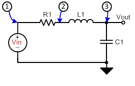
Netlist
V_1 1 GND Vin
R_1 1 2 R1
L_1 2 3 L1
C_1 3 GND C1
VOUT 3
VIN 1
Netlist
V_1 1 GND Vin
R_1 1 2 R1
R_2 2 3 R2
OPA_1 GND 2 3
VOUT 3
VIN 1
Netlist
V_1 1 GND V1
V_2 2 GND V2
V_3 3 GND V3
R_1 1 4 R1
R_2 2 4 R2
R_3 3 4 R3
R_4 4 5 R4
OPA_1 GND 4 5
Netlist
V_1 1 GND Vin
R_1 1 2 R1
R_2 2 3 R2
C_1 2 3 C1
OPA_1 GND 2 3
VOUT 3
VIN 1
PoleZero_
The second feature to take notice of is the 'PoleZero_" option. When this is set the program will solve for any poles and zeros in the system. An example output would be the below:
The 'PoleZero_' option works for both symbolic and real values, and even a hybrid mixture of the two. This is shown in the netlist below.
Netlist
V_1 1 GND Vin
R_1 1 2 50
R_2 2 3 100
C_1 2 3 1e-9
OPA_1 GND 2 3
VOUT 3
VIN 1
PoleZero_
The output would be the below:
Netlist
V_1 1 GND Vin
C_1 1 2 C1
R_1 2 3 R1
R_2 3 4 R2
OPA_1 GND 3 4
VOUT 4
VIN 1


No comments:
Post a Comment